Aesthetic Stats: Mean Minus One (MM1)
Mar 18, 2020 00:00 · 1846 words · 9 minute read
"If you want to make God laugh, tell him about your plans.
I simply planned to go to and from my work at UCL to explore the neural mechanism underlying aesthetic experiences while watching as soggy London transitioned into spring. I also planned to go back and forth to my home, in Italy. Instead, I recently found myself “stuck” in the house, with some spare time and a lot of work that I decided to postpone. So here I am.
INTRO
Since basically I am applying the MODIFIED POMODORO method to my working schedule (see thread below), I decided to come up with some “tutorials” on how to compute useful metrics for aesthetic science.
now that we are all working from home, may i recommend:
— Dr. Caroline Bartman (@Caroline_Bartma) March 16, 2020
the MODIFIED POMODORO method.
1. work on work stuff for 25 minutes.
2. Read coronavirus updates on twitter and https://t.co/LQmVJPrqWd for two hours
repeat until you've finished approximately 25 minutes of work in 1 day
In this article, and maybe in a couple later, I will use the powerful resources that are out there (open access data), to create useful tools for researchers in the field of aesthetic science. The first metric I will describe is Mean Minus One (MM1), which is a tool to measure agreements across individuals. The MM1 is a tool used extensively by Edward Vessel 1, and it is a sort of more unbiased pairwise cross observer correlation. Shortly, MM1 gives you a number that quantifies how much individuals score kind of the same on a set of Items. For example, Vessel used MM1 to quantify how much individuals agreed on aesthetic ratings of faces (spoiler: a lot), landscapes, architecture (both interior and exterior), and abstract artworks (spoiler: not so much).
Here, for the sake of open science, reproducibility, and because I finished all the Ghibli’s masterpieces on Netflix I will:
- Show you how to compute MM1
- Try to reproduce Vessel’s results
- Create some nice data Viz of agreement
hopefully, at the end of this tutorial, you will know how to test by yourself if your participants agreed on a certain topic (whatever agreement on a certain topic will mean in your study, i.e. agree on aesthetical pleasantness) in a given domain (again, whatever domain will mean for you, i.e. faces, landscapes, …).
HOW TO COMPUTE MM1
(adapted from this article 2). What you need is a data frame (df), with Subjects ID in the first column, and Items (the thing we use to measure what we want to measure) in the other columns. So you will have all the scores for one participant in one row (wide format). In the case of Vessel 2018, one df will have People ID (coded) on the first column, different faces on all the other columns, and ratings of aesthetic pleasantness (in this case a measured with a 1 to 7 scale) in each cell. N.B. one df is representative of one domain (i.e. faces).
Below you have an example of the transpose df. You don’t need to have that as the function will already swap rows and columns. But for the sake of the readability of the instruction in the next section, here you have a snapshot of a fraction of a df:
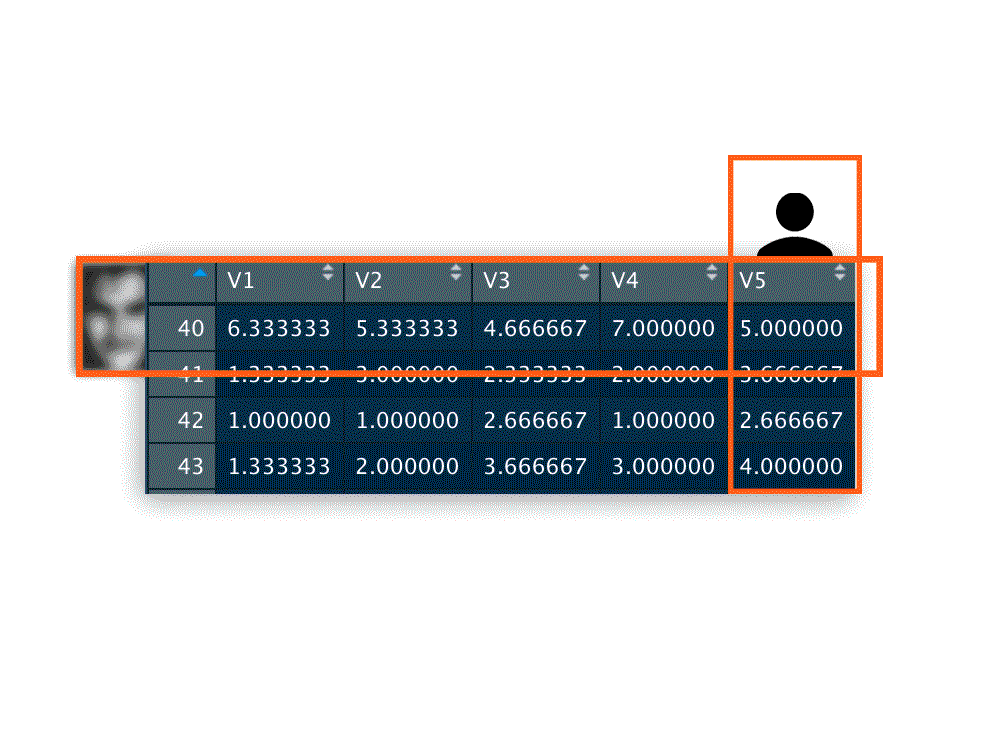
Row = Items ratings (yep I blurred the face). Column = Subject ratings. As you can see, there is some agreement on how aesthetically pleasing the item is on row 40 (Participants to this study rated that face quite high)
Now if you have a df like the one I specified above (for the specialist, there shouldn’t be NA in the dataset, as the function I wrote doesn’t handle missing stuff), you can use this function:
#Mean Minus One.
#Create a function that given a dataframe with rows as Subj and Column as Items compute the MM1.
#Requirments: tidyr Package, no NA, subj ID on the first column.
#Coded by: Giacomo Bignardi

library(tidyr)

MM1 = function(df){

  #transpose the df
  df = t(df)
  #save subj id
  id = df[1,]
  #remove subj id
  df = df[-1,]

  #Compute means minus ones
  means = matrix(0, ncol = ncol(df), nrow = nrow(df))
  for(j in 1:ncol(df)){
  mean = c()
    for(i in 1:nrow(df)){
      mea = mean(as.numeric(df[i,-j]))
      mean = c(mean,mea)
    }
  means[, j] = mean
  }

  #Compute correlations between means minus ones and ones ratings
  mm1 = c()
  for(j in 1:ncol(df)){
  cor = cor(df[,j],means[,j])
  mm1 = c(mm1,cor)
  }

  #transform correlations into z scores (r to z Fisher)
  zScores = c()
  for(k in 1:length(mm1)){
    z = (log((1+mm1[k])/(1-mm1[k])))*0.5
    zScores = c(zScores, z)
  }

  #save average correlation (z average to r average Fisher) and correlations per Subj
  MM1List = list((exp(2*(mean(zScores)))-1)/(exp(2*(mean(zScores)))+1), cbind(id,mm1))
  names(MM1List) = c("MM1", "summary")
  MM1List
}
Done.! If you want to follow step-by-step what the function does read down below. Otherwise, skip the next paragraph and look directly at how you can interpret the MM1.
1) it transposes the df. That is, it puts subjects as columns and items as rows (as in the image above). This is needed to make calculations feasible;
2) it deletes (and store somewhere else) the ID number (we do not need ID numbers to compute MM1;)
3) It computes the mean score for each object (now each row) from every subject ratings except for one subject. It iterates such process for every other subject (wait, what? Means minus one. Lol; )
4) it computes the correlation between the ratings of subject removed and the means minus one (mm1r). It iterates such a process for every other subject;
5) It convert the correlation scores to z scores;
6) it compute the average of the z scores;
7) Convert z - to - r again.This final averaged r is our MM1.
This MM1 can be interpreted as a measure of agreement. MM1 near to 1 means that almost everyone agrees. In our case (Vessel et al. example ()) it would mean that everyone reported the same degree of aesthetic pleasantness from the same faces. On the other end, MM1 near to 0 means that almost everyone disagrees, which would mean that everyone reported very different aesthetic responses to the same faces.
REPRODUCE VESSEL’S RESULTS
Now that we have a function to calculate mm1r and MM1 we can try to replicate the results of Vessel et al. The nice thing about open access is that we can directly play with the data :). You can find the data of Vessel here. Before running MM1 we need to prepare the df. The following code will do it for you.
#example of comparison
#Requirments: readr, dplyr Packages, MM1 function

library(readr)
library(dplyr)

#load dataframe (just download the dataframe from https://edmond.mpdl.mpg.de/imeji/collection/dMlhGcI642YmIIF2 and put them in your desktop)
Vessel2018_faces <- read_delim("data_2020_03_18/Vessel2018_Agreement_Exp1_fac_20ss_rating_LONG (1).txt", #directory and name of the file
                               "\t", escape_double = FALSE, col_types = cols(Block = col_number(),
                                                                             Image = col_integer(), RT = col_number(),
                                                                             Rating = col_integer(), Subj = col_integer(),
                                                                             Trial = col_number()), trim_ws = TRUE)
#Select the important variables (SubID, Items and ratings)
Vessel2018_faces = Vessel2018_faces %>%
  select("Subj","Image","Rating")

#take the average of ratings per repeated images (this steps is not necessary if you don't have multiple scores on the same Item)
face = Vessel2018_faces%>%
  group_by(Subj,Image)%>%
  summarise(Rating = mean(Rating))

#Create a Wide Format (required)
faceWide = spread(face,"Image", "Rating")
Once df is ready, all you need to do is calling the function:
#compute MM1
faceMM1 = MM1(faceWide)
MM1 for faces is 0.84. Pretty similar to the one reported by Vessel! Great, We reproduced Vessel’s 2018 results! Pretty cool. This means that, in this sample and with this set of images of faces, the aesthetic agreements between participants is pretty high. That is, people seem to strongly agree when they are evaluating faces.
NICE DATA VIZ OF AGREEMENT
What if you want to compare 3 more than one domain? First you can just replicate the same procedure for other domains, such as images of landscapes, internal and external architecture, and artworks. One possible way to interpret the data is to just read the MM1. However, given that MM1 is kind of an equivalent to the mean of the distribution of the mm1r, it would be better to find a way to visualize the result by showing as much relevant information as possible. For example, what about individual agreement vs. general agreement? Below, you have an example on how we can visualize the results, to get a grasp on the differences between domain while not losing information about the individuals. F irst, we need to repeat the same thing as for faces. I did it, but I will not show you the code, as you can repeat exactly what I did before with faces! Tips: first download the data from here.Then remember to adapt the directory to load the file in R-Studio.
An important step to do after you computed and stored the MM1 lists is to create the proper variables required to create the graph. This might be a bit annoying, so here you have the code:
#Convert mm1r to dataframe (required to plot them)
faceAgreement = as.data.frame(faceMM1$summary)
arcExtAgreement = as.data.frame(arcExtMM1$summary)
arcIntAgreement = as.data.frame(arcExtMM1$summary)
lscAgreement = as.data.frame(lscMM1$summary)
artAgreement = as.data.frame(artMM1$summary)

#Create and additional column with the name of the domain
faceAgreement$domain = rep("face", nrow(faceAgreement))
arcExtAgreement$domain = rep("architecture_Ext", nrow(arcExtAgreement))
arcIntAgreement$domain = rep("architecture_Int", nrow(arcIntAgreement))
lscAgreement$domain = rep("landscape", nrow(lscAgreement))
artAgreement$domain = rep("art", nrow(artAgreement))

AgreementPlot = rbind(artAgreement[,-1],arcIntAgreement[-1],arcExtAgreement[-1],lscAgreement[,-1],faceAgreement[,-1])
#convert to factor the domains
AgreementPlot = AgreementPlot %>%
  mutate( domain = factor(AgreementPlot$domain, levels = c("art","architecture_Int","architecture_Ext","landscape","face")))

#Create a dataframe to represent the MM1 as line in out graph
MM1_lines <- data.frame(domains = factor(c("art","architecture_Int","architecture_Ext","landscape","face"), levels = c("art","architecture_Int","architecture_Ext","landscape","face")),
                         x0 = c(as.numeric(artMM1$MM1), as.numeric(arcIntMM1$MM1),as.numeric(arcExtMM1$MM1),as.numeric(lscMM1$MM1),as.numeric(faceMM1$MM1) ))
Finally, we are ready to plot the graph:
library(ggplot2)
library(ggridges)


ggplot(AgreementPlot, aes(x = mm1, y = domain, fill = stat(x))) +
  geom_density_ridges_gradient(jittered_points = TRUE,alpha = .95,
                               size = 0.2, point_alpha = 0.5, scale = 1.1) +
  geom_segment(data = MM1_lines, aes(x = x0, xend = x0, y = as.numeric(domains),
                               yend = as.numeric(domains) +1), color = "black",size = 0.5, alpha = 1) +
  scale_fill_viridis_c(option = "plasma", name = "mm1") +
  scale_x_continuous(limits = c(NA, 1)) +
  coord_fixed(ratio = 0.2) +theme_ridges(grid = FALSE)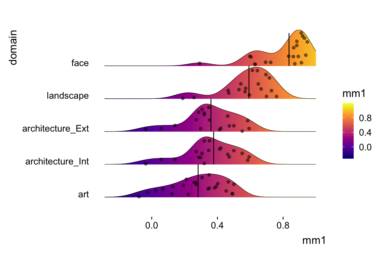
Ok. Done! the color gradient represents the intensity of agreement. The brighter, the higher the agreement. The dots represent the individual mm1r, that is individual’s agreement to the mean. The blackline at the “center” of the distributions marks the MM1 for the domain (slightly different from the mean of the distribution.) By looking at art and face domain, for example, we can see that agreement for art seems to be lower than for faces, and that individual agreement seems to vary more for art than for faces (it almost looks like there are two clusters of agreement in the face category).
That’s pretty much all. Feel free to use the code and make it better. But please, if you spot some errors send me a tweet. Ciao
Vessel, E. A., Maurer, N., Denker, A. H., & Starr, G. G. (2018). Stronger shared taste for natural aesthetic domains than for artifacts of human culture. Cognition, 179, 121-131.↩
neuroaestheticsandcreativity.net/post/the-subject-s-at-the-center-of-aesthetic-experience↩
To compare different domain we would actually need to run an ANOVA.We will not, as it is not the aim of this tutorial.↩